Imitating Fund Managers using GANs
A chapter from the thesis The Market as an Ecosystem
Species of Investors
Introduction
Investment strategies vary widely in their objectives, styles, management and execution. Understanding these strategies is essential for practitioners, regulators, and researchers investigating asset pricing and market dynamics. Traditional classifications, like those provided by Morningstar and Lipper, rely on broad style categories. While useful, these methods often fail to capture the complexity of real-world portfolios and the underlying trading strategies. A detailed understanding of portfolio management to the level of implementation is necessary in order to be able to realistically simulate financial markets in, for example, agent-based models.
This chapter builds on the factor model introduced in Chapter 3 to characterize long-term investment strategies through a combination of data analysis, risk-factor modelling, and representation learning.
Motivation
In the overview of different models of thinking in Chapter 2, Sections 2.1-2.5, we investigated models of rational behaviour and models of classical finance. We question how these models translate to the real world, and how we identify investment strategies in the data. This directly answers Research Question 1 (Section 1.3).
We want to understand whether this regulatory filing data, that is made publicly available with the express purpose to make investors gain trust in financial markets, is sufficient to really understand what managers do. This combined work, of data analysis and bottom-up strategy replication, allows us to get a better understanding of how these funds manage their portfolios and allows us to systematically learn how to construct and manage such portfolios.
Overview of Existing Methods
Our approach is motivated by a survey of existing work on classifying the strategies and styles of investment funds, which we summarise in Table [table:classification_schemes].
Surveying all the methods in Table [table:classification_schemes], we find that most approaches are easily replicated, with the exception of Morningstar’s categories where the white-paper is unclear details to replicate the exact results, and the MSCI methods which are proprietary. Selecting only those schemes that we can replicate on our universe of U.S. equities, the Lipper scheme is the most comprehensive: due to its larger amount of factors it includes other models. On top of this, the Lipper database also provides the stated objectives of funds from prospectuses, and so it provides additional insight into the managers’ intentions.
Limitations of Existing Fund Methods
Characterisation of the portfolios requires addressing several aspects: the exposure of the portfolio to the risk factors as the investment style, the use of borrowing or leverage, how these exposures compare to peers with the same stated objectives, optimising behaviour, the stability of the of the investment style, and learning to trade from reconstructed portfolios. All of these aspects have the potential to affect future returns. While top-down approaches, which correlate funds’ returns with known index portfolios constructed in the same universe [@Sharpe1992AssetAllocation; @Hasanhodzic2007CanCase], can characterise funds’ risk-factors reliably, they do not reveal whether a fund optimises or uses leverage and how they manage risk in a way that results in a full replication of the strategy. Although the predictive power for future performance of the ranking systems built on top of the style classification is rather limited (see, e.g., [@Blake2000MorningstarPerformance]), an empirical observation in fund management is that investors make investment decisions based on historical performance within style peer-groups [@Chevalier1997RiskIncentives], thus underscoring the importance of accurate grouping.
When the Carhart model is used as the ground truth for risk factors in a portfolio, 14% of funds are found to be misclassified between 2003 and 2016, according to [@Bams2017InvestmentPerformance]. Market dynamics may lead to investments migrating from one category to another, faster than the manager can adjust their portfolio leading to tracking error. In reviews of existing classification systems, it is found that historically significant numbers of mutual funds are incorrectly classified due to these combined effects [@Kim2000MutualMisclassification]. In the literature on mutual funds, researchers have discovered individual cases of portfolios moving away from stated investment objectives, and the multiple reasons for why this may happen fall under the term of [@Wermers2012MatterPortfolios].
Modelling multiple opponents in an adaptive, non-stationary game can be effectively approached by learning deep representations, as demonstrated in dynamic, multi-agent reinforcement learning settings [@He2015]. These methods highlight that high-dimensional data describing the actions of players or agents can be effectively encoded and represented using deep neural networks. Such representations allow the model to generalise across varying strategies and adapt to changing dynamics. Learning in a continuum of opponent strategies may be an advantageous setting, as in practice opponent modelling still performs well when presented with mixtures of pure opponent strategies the learner is already familiar with [@Smith2020LearningOpponents].
Many settings in the opponent modelling field assume interaction between the learner and the opponent agents. These settings are often explored in simulation because then the learner can better explore agents’ behaviours by adjusting its own actions. Regulatory reporting data is static and not as abundant as the number of evaluations of a simulation, and so there is a risk of overfitting, where the learner does not generalise behaviour but only recalls individual responses in specific contexts.
A class of neural networks called generative adversarial networks (Section 1.3.4.1 for a discussion) have been used to extend real data with realistic synthetic data, to enhance training of downstream tasks such as trading strategies [@Eckerli2021GenerativeOverview]. They have been applied in the context of portfolio management [@Mariani2019PAGAN:Networks] to better model the dynamics of the underlying instruments in a Markowitz-style framework, on top of which a trading strategy then can be tested.
We can however model the dynamics of the financial instruments through our factor model, and so our focus shifts more towards learning representations for the observed strategies in the data.
In the literature of generative models, it is often the case that the exact criteria for replicated behaviours to be realistic is hard to define, but these can be learned in a competitive setting between generator and discriminator [@Goodfellow2014GenerativeNetworks]. The use of discriminators in the loss function means the network can implicitly learn what defines a certain strategy, and so it doesn’t need to rely on an exhaustive list of criteria relevant to classify a strategy.
Objectives
The main objective of this chapter is to gain a thorough understanding of investment strategies, that is both practical – in that it allows us to simulate realistic investment funds, as well as comprehensive – in that we can relate it to the theoretical frameworks of academic finance.
We analyse portfolios based on their typical risk-factor exposures, their alignment with benchmarks, and their adherence to mean-variance optimisation principles. This characterization provides an operational understanding of fund strategies beyond labels. We want to validate our classification by investigating the stability of the exposure-based classification for major funds, for which we have long periods of holding data.
Having decomposed returns into constituent risk factors in Chapter 3, we briefly revisit the factor model to analyse the risk factor exposures at the portfolio level in order to understand the composition of portfolios of different styles in Section 1.2.3. We compare these classifications to the existing Lipper style-score methodology. In the diagram of Figure 1.1, we display the various aspects of portfolio management discussed in this chapter, and we link to the sections that discuss these separate topics.
Operational Objectives
Our objective when learning strategies from data is to learn a latent representation of portfolio behaviour directly from the portfolio data triple , meaning the characteristics of the investments, the returns , and the weights . The latent representation for one fund manager is fixed to a small number of variables whereas the decoder needs to be able to deal with variable numbers of stocks and long histories of the time series of the returns .
Formally, we model the conditional probability:
where is a low-dimensional latent variable specific to manager ’s strategy.
In order to learn strategy representations for real-world funds, we extend our factor model with a strategy classifying component and a discriminator. These will be discussed in Section 1.1.2.1.
Holdings-Based Investment Strategy Analysis
In this section, we outline the methodology used to characterise real-world portfolios, determine their strategy and make a classification, evaluate the stability, and derive portfolio-management and risk management components from the data.
Identifiability of Strategies
We identify two important aspects of portfolio processes that can be directly calibrated to regulatory reports. The first are positions at a point in time, which are captured in so-called holdings reports. The second aspect are the dynamics, which are more difficult to characterise but for which we have such statistics as the turnover rate that we can directly use in calibration.
Reconstructing Positions in Time
Markets are open to trade most business-days of the year. However, we only have holdings data at most at a monthly frequency. There also exists uncertainty about the precise moment in time to which the portfolio applies for the following reasons. Regulators typically ask for the last reporting period date and allow the fund manager to pick the nearest preceding business day so that the manager can use actual market prices to value their portfolio. However, markets worldwide adhere to different calendars, meaning some of them will be closed, and therefore the view on the portfolio may not be consistent. On top of this, we frequently encounter stale data in the reports. Hypothetically in cases where an instrument’s price does not cross the same reported price more than once, we can determine that the market prices used in the report must be several days or weeks older. However, prices are volatile, making it impossible to automate correcting these errors.
Trading Signal Frequency
The data constraints described in Section 1.2.1.1 make identifying the dynamic strategies difficult, as their frequency is much lower than that of the signals in market data that may influence the portfolio choice. The low frequency of portfolio holdings reports means that if a fund manager trades frequently, we cannot fully reconstruct their strategy. We ask whether there exist some methods to inform us about how much we can reconstruct
The Nyquist-Shannon sampling theorem tells us that, to fully resolve a frequency-limited signal, we need to sample at a rate of at least twice the highest frequency in the signal. When we sample at a frequency less than the highest important frequency of the trading signal, we cannot accurately recover the signal and instead up with a signal alias, which not only is likely to have a frequency that is much too low but may in rare cases also result in complete loss of the signal. Suppose the manager buys and sells the same instrument in a given period between the known reports at time points and . We only observe the net position that resulted from these trades at time . If an investment strategy depends on signals that are a higher frequency than twice our monthly holdings positions, we are downsampling, and we may mischaracterise those strategies. We expect this to be the case for strategies that depend on high-frequency indicators, such as technical trading strategies that derive their signal from market prices and volumes, such as momentum strategies. On the other side, fundamental strategies based on slow economic indicators, such as the firms’ earnings reports, have a natural frequency of a quarter year between data points and are therefore resolvable.
Specialist financial entities such as market makers are known to only hold positions for brief periods, rarely maintaining risky positions between market sessions or over the end of a reporting period [@KIRILENKO2017]: we cannot model strategies that rely on clever order placement and intraday positions, such as high-frequency market makers and arbitrageurs. We do not observe the individual trades, nor the details of the orders submitted to a market to engage in those trades. For these reasons it is unlikely that we will be able reconstruct meaningful strategies for these types of financial market participants, and hence our focus shifts to long-term investment funds such as mutual funds.
Data and Coverage
We use institutional portfolio holdings data and U.S. equities’ market data as the basis for this study. We re-use the risk-factor exposures or loadings from Chapter 3(this equation). The holdings data represent positions at the portfolio level. The data is updated at, depending on regulatory regime and voluntary public disclosure, quarterly to monthly intervals. As data quality and coverage constrains our analysis, our primary investigation uses a commercial compilation of cleaned up public reports at the portfolio level. These are obtained from the CRSP Survivor-Bias-Free US Mutual Funds database[@CRSPPrices], based on the work by [@Wermers2000MutualExpenses]. Portfolio-level data in the format of the Securities and Exchanges Commissions’ forms are essential to our risk-factor exposure based classification. Aggregation at the level of a financial firms prevents us from doing a reliable strategy classification, though that is the case for other forms such as . In light of research in later chapters (Chapter [chapter:hypothesis]) where the total holdings explained through regulatory reports become important, we do a more extensive investigation into public regulatory filings at the legal entity level in Appendix A.
We narrow down out data to periods and portfolios that have good coverage. We define the threshold to be that 75% of the market value of the portfolio must be explained by our factor model, meaning for that portion the factor loadings are reliably estimated. A portfolio also must have at least one year’s of observations, and over the period it is observed at least 75% of the time it must have complete data. To make comparison possible, we also select those funds that have a classification by an existing classification system, in this case a Lipper class (classifying the fund in the wider mutual fund landscape) and a Lipper objective code (categorising the objectives set out in the prospectus).
Compared to the financial instrument data, we have a relatively short span of high-quality portfolio data with wide coverage. Accordingly, in this chapter, we fit models using data from 2010 to 2018 and validate them using data from 2019 to 2022. For qualitative analysis, all visualization samples are drawn from December 31, 2019. This date marks the end of the year, which for many firms marks also the end of a fiscal year and coincides with an annual report, which is typically when numbers are most accurate. This date in 2019 is the month with the highest number of complete portfolio reports, providing the richest dataset for visualisation.
The Fund Balance Sheet
We denote by the weight of an investment in the portfolio at time . In the reports, the weight is officially the allocation fraction of total net assets, and is computed by the fund using the appropriate accounting methodology. In rare cases where the investment is recorded but the percentage is not provided, we recompute them using mark-to-market accounting if other values such as the number of contracts or the notional is provided. In older reports, mainly before the 2000s, the specification demanded human-readability of the documents, and in such cases numbers are often rounded leading to many investments receiving a zero weight. In such cases we also recompute the weight using mark-to-market valuation. If the (TNA) of a fund are defined as:
then, the allocation fraction for instrument can be computed as:
The portfolio allocations or portfolio weights tell us what fraction of total net assets is invested in a certain instrument. The weight can be negative, when the instrument represents a liability such as a short position.
Style Classification
In this section we discuss the benchmark methods to which we compare our approach. As discussed in the Motivation (Section 1.1.1), we settle on using the Lipper Style Classification methodology as the benchmark, as we can replicate it closely.
Projections of Portfolios on Factors
Motivated by our intent to classify portfolios using only those factors that explain returns, in this section we explore the direct projection of the investment portfolios on the (latent) factors uncovered using the deep learning model in Chapter 3.
In subsection 1.2.3.2, we discuss the expectations we have about applying factor models to portfolios in the theoretical framework on which the model is built. We then relax these assumptions and consider which other aspects of portfolios we might want to capture, in Subsection 1.2.5.
Factor Models applied to Portfolios
Recall the factor model of instruments’ returns in this equation, and the allocation vector being the weights of the instrument in the portfolio at time (this equation). We expect that the log return of the portfolio , as defined by the allocation fractions is:
In the model, the residuals are independent, therefore decreasing the concentration of the allocations leads to . Whereas the risk-factor sensitivities lead to a dependency on shocks in the risk factor which aggregates over all holdings in the portfolio, the residuals vanish in expectation as the weight assigned to any one instrument becomes small, . It is expected that when explaining the cross-section of the returns of investment portfolios, the explained variance is at least as good on average as explaining the cross-sectional variance of individual financial instruments. But furthermore, we expect that the explanatory power increases much further, due to diversification.
When it comes to the style of a portfolio, it may be useful to think of the portfolio in terms of its mean exposures, as the mean exposure times the factor shock represents the direct contribution of factor to the returns, at time .
The vector of values for all risk factors is a simple statistic that is often used to compare portfolios’ investment styles, and hence is called the .
Lipper Classification Methodology
The Lipper Global Holdings-Based Classification[@1999REFINITIVMethodology] is a system for grouping mutual funds of multiple asset classes. The methodology is broad and covers both equity and fixed income funds, but we focus on the equities portfolios here. The investment style component of the model comprises a scoring scheme taking a moving average with the weighted score of up to 6 recent portfolios, with more weight placed on recent portfolios.
Reference Index
The Lipper scheme uses the Russel 3000 index as the benchmark index for U.S. equities. The historic index constituents are available as a data product from S&P Global, but the rules for candidates to be included are simple enough that we reconstruct our own reproduction of the index and its historic statistics (Appendix A).
Lipper Model Steps
Stock market cap size classes are fixed: small, mid, large. The boundaries between these classes are evaluated every June. Large cap stocks are the stocks with the largest market capitalisation that combine to have 40% of the total market capitalisation. The next largest stocks that combine to an additional 30% of the total are the mid cap stocks, and the remainder up to and including the rank-3000 largest stock are the small cap group. Roughly speaking for US equities funds, if a fund’s holdings are at least 75% in one class, they belong to that size class, and otherwise they are labelled as being multi-class.
Next, the instruments in the portfolio are scored according to weighted sum of scores on the individual factors. For each factor, the market capitalisation weighted mean and standard deviation for the benchmark index are computed.
Then, for each portfolio, the allocation-weighted average score is computed for each factor as the z-score of the portfolio mean to the benchmark index mean and standard deviation, simply . When historic portfolios are available, an exponentially weighted moving average according to the weights is given in appendix Table 1.1.
The style score is then the sum of the scores on individual factors. The first three factors contribute towards the instrument counting as a growth stock, the latter three factors are associated with value investments. Each factor is sub-scripted to indicate these are computed according to the Lipper specification, as other variants may appear elsewhere in the text.
| Weight | Factor | Compustat Variables |
|---|---|---|
| +1 | price-to-earnings | |
| +1 | price-to-book | |
| +1 | price-to-sales | |
| -1 | return on equity | |
| -1 | dividend yield | |
| -1 | 3-year earnings growth |
- This table lists the six variables in the Lipper Style Score model, and the Compustat variables used to compute them.
The scores are computed for all the instruments in the benchmark index and instruments that are not in the index but that appear in the holdings of the portfolios alike. Later in this chapter we will give the models the most recent and older portfolios to learn from. Therefore it is not necessary to compute the weighted moving time average, as even the linear models should be able to learn a weighting scheme of current and historical values.
Leverage Ratio
The is defined as the ratio of risky instruments to the net asset value .
The choice which instruments are considered risky and which are safe depend on the firm and the jurisdiction they operate in. Usually, these instruments are cash (currency) or sometimes high-quality (government) bonds are included.
Therefore, in our most general specification we define a set of safe instruments. As we continue our focus on US investment funds, in practice, this set contains only US Dollar cash, short-dated US-government securities such as treasury bills, and any amount participating in money market funds. The relationship between the allocation fraction, leverage ratio and portfolio net value is:
In the case of Form 13F we do not have all balance sheet items available. As in many reports the allocation weights are omitted and the total asset value is not stated, we do not know the leverage ratio, and we must assume that the leverage ratio . This is not the case for Form N, and specifically Form is highly detailed: not only are all accounting values mandatory, we also get a breakdown of assets considered to be part of the safe assets .
Portfolio Optimisation
While the factor projections of portfolios suggest that managers often coordinate on stable combinations of risk exposures, this is not enough to explain all portfolio weights in the data. This is clear from inspecting the portfolios of various funds for which we have reliable style classifications aligned with the stated objective in the prospectus: it is clear that for many funds there are cases where a monotonic preference relationship between risk-factor exposure, market capitalisation, and the allocation weight in the portfolio is violated. This indicates that portfolios are further shaped by processes beyond the constraint on a certain investment style.
In the literature, the focus is often on expected returns (the first moment) and return volatility (the square root of the second central moment). As discussed in Chapter 3, under the assumption of market efficiency (Appendix A), the market reflects a single price for a unit of volatility. This does not preclude heterogeneity in the preferences of investors when it comes to the reward-risk trade off.
The foundational work of Markowitz [@Markowitz1952] introduced the framework for portfolio optimisation by balancing expected returns against risk, where risk is quantified as portfolio variance. This approach forms the basis of modern portfolio theory and later inspired Sharpe’s [capm]{acronym-label=”capm” acronym-form=”singular+short”} [@Sharpe], which further formalized the relationship between expected returns and market risk through the concept of the market price of risk.
A common optimisation goal in this framework is to maximise a utility function that incorporates both return and risk, parametrised by a risk-aversion factor
Where represents the weight of asset in portfolio at time , and is the return of asset at time . This equation generalises Sharpe ratio maximisation and incorporates flexibility for varying risk preferences. Figure 1.3 illustrates these concepts: the curved arcs represent all portfolios that are optimal in terms of this equation for different choices of risk-aversion . These curves as parametrised by are called the . In this diagram, we observe two frontiers: one efficient frontier for portfolios on all possible instruments in the market where the style of the portfolio is unconstrained, and one for all portfolios that satisfy the style constraint. The diagram illustrates that the constraint of having the mean portfolio exposures near a target style, makes the set of valid portfolios smaller, and makes it likely that constrained portfolios have lower expected returns or higher volatility than unconstrained optimised portfolios, or both.
In the confines of the Markowitz framework, speciation or the constraint to a certain investment style, thus seems irrational, as a wider investment universe likely permits optimised portfolio combinations with higher expected return, lower expected volatility, or both, with the exception of the case where the stock portfolio constrained to a certain risk exposure serves to offset risks the investor is exposed to in other types of investments or income streams.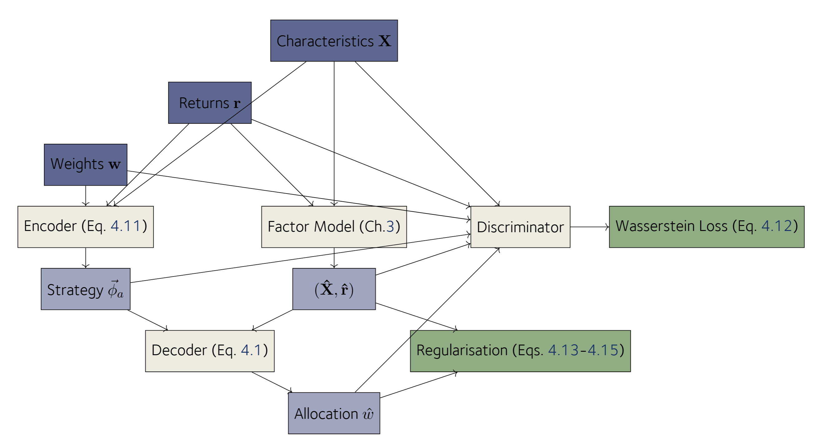
As came up in the investigation of factor model optimality in Chapter 3, Section [section:residual_alpha_information_criterion], a condition for optimality of a portfolio is that the joint alphas defined as the idiosyncratic returns of all assets relative to the portfolio are zero [@Gibbons1989APortfolio]. However, testing this in practice is challenging due to the low statistical power of such tests in limited datasets, where estimation errors for variances and covariances can dominate. Furthermore, real-world instruments often exhibit significant idiosyncratic returns, reflecting deviations from market efficiency caused by transaction costs, liquidity constraints, or behavioural biases. Some fund managers also demonstrate persistence in returns [@Carhart1997OnPerformance], suggesting that alphas may not always align with theoretical expectations. Given these challenges, we choose not to perform these tests directly. Instead, we adopt a more general optimisation test that allows for the inclusion of additional constraints in this chapter in Section 1.3.3.
Turnover Rate
As discussed in preceding Sections 1.2.3-1.2.5, the dynamics of both the underlying economic variables and those of market prices themselves cause the portfolio to drift away from the desired allocation. Thus a manager may need to actively intervene by trading the instruments in the portfolio.
We adopt the absolute turnover metric (this equation) to quantify portfolio trading activity because it captures the volume of capital reallocated through buying and selling, normalised by the portfolio’s net value. This measure is particularly suited for evaluating operational costs and market impact, as these arise from any trading activity, regardless of its purpose. Unlike metrics that focus solely on relative changes in portfolio composition (See a discussion in Appendix A), absolute turnover also accounts for trading driven by fund flows, such as investor deposits or withdrawals, which can represent a significant fraction of overall trading activity. By including all sources of trading, absolute turnover provides a practical assessment of the trading intensity associated with the strategy. Additionally, normalising by the portfolio’s net value ensures comparability across portfolios of different sizes.
The turnover is defined as:
In this definition, are two points in time at which the positions of the portfolio are observed, and are the year fractions used to annualise turnover rates. The constant two appears in the denominator as a full turnover cycle of the portfolio is defined as the building up of a position and winding it down, thus leading to twice the observed trading quantity.
Experiments
In this section we detail the initial experiments investigating classification stability (Section 1.3.2), portfolio optimisation (Section 1.2.5) and
Model Alignment
In this section, we perform the model alignment and comparison with the Lipper methodology focusing on the investment styles. We first need to make the model comparable, by putting them in same coordinate
Procrustes Analysis
In order to be able to compare the latent factors uncovered by our neural network and the explicit factors of the Lipper methodology, we need to align the spaces these methods span. Specifically, we want that the average factor loadings of portfolios grouped by Lipper class is aligned with the average of the same portfolios
A family of methods called Procrustes analysis offers the tools to perform this alignment (a comprehensive summary can be found in [@Gower2004ProcrustesProblems]). In our case, we are looking for a transformation matrix such that the dot product of the factor model is maintained, essentially meaning that our prediction of is not affected by the transformation of the latent variables:
This is known as the orthogonal procrustes problem [@Schonemann1966AProblem] and can be solved by making an orthogonal rotation matrix, meaning solutions have . For all Lipper labels , we take a set of portfolios that are observed over the entire period so that the statistics aren’t influenced by portfolios coming in to the sample and leaving. We compute the mean exposure for each label . Next, want to minimise the distance of the time difference:
where the Frobenius-norm squared means we are minimising the sum of all elements squared. [@Schonemann1966AProblem] showed that taking the singular value decomposition of the product of the means of each label gives the solution .
Model Equivalence Testing
We move ahead with the projection of the portfolios onto the factors that we found when explaining the cross-section of the returns of US equities, aligned by For all funds in our data where we have computed an average factor loading , we have Lipper classifications. We focus on investment style aspect of the classification, and take the Growth and Value orientation of the funds. We perform the following test to see whether our factor model is aligned with the Lipper classification scheme.
To test the compatibility of our factor model with the Lipper classification, we assign class labels of +1 for Growth, -1 for Value, and 0 for Core funds. Factor loadings are used as input features for a Support Vector Machine (SVM) to find linear decision boundaries.
The data is split into training and test sets, with 50% reserved for each. Results are summarised in Table 1.2. The first panel shows performance for Growth and Value styles, and the second includes the Core class. Between Growth and Value, classification accuracy is 97.3%. Including Core reduces performance due to greater overlap in factor space, suggesting a more complex structure in the latent space that the linear SVM cannot fully capture.
| Panel A: Growth vs. Value | Accuracy | Recall | F1 Score |
|---|---|---|---|
| Value | 0.984 | 0.973 | 0.978 |
| Growth | 0.955 | 0.974 | 0.964 |
| Average | 0.973 | 0.973 | 0.973 |
| Panel B: Growth, Value, Core | Accuracy | Recall | F1 Score |
|---|---|---|---|
| Value | 0.817 | 0.868 | 0.842 |
| Core | 0.746 | 0.688 | 0.716 |
| Growth | 0.923 | 0.876 | 0.898 |
| Average | 0.838 | 0.837 | 0.837 |
- SVM classification performance linking factor model classifications to Lipper’s investment styles. Panel A reports results for Growth and Value styles only. Panel B includes Core styles.
We observe that when it comes to the three typical categories relating to style, obtain an approximate 83.8% commonality, as read from Table 1.2 for the accuracy of the three-label variant in Panel B. On average there is 16.2% discrepancy, which is close to the discrepancy reported in the literature when using different factor models as the ground truth, such as the Carhart model [@Bams2017InvestmentPerformance].
Diversity of Risk Factors
Do fund managers have subjective ideas about what constitutes a certain investment style? We investigate pairs of funds that share the same management company. For all management firms that manage both a value and growth fund on the same universe, we compute the difference:
where value, growth are the portfolios of fund manager and are the portfolio average exposures to risk factor .
We expect that if all managers follow the same interpretation of the risk factors, then the vectors all point in the same direction. We can efficiently test this by taking the mean vector over all managers, and computing the cosine similarity between individual manager’s vectors and the population mean. We expect that this is especially the cases for the risk factors that show a clear and steady separation between the means of the different classes as demonstrated in Section 1.3.1.1. This is not the case in aggregate: only the risk factor that receive the highest importance in the factor model have positive cosine similarity for all managers. There, the average cosine similarity to the population average is 0.599, indicating high similarity in the beliefs management firms have about the orientation of an investment style in factor space. When other risk factors are included such as the market factor, 42.2% of managers in fact have a negative cosine similarity, indicating high diversity among the other risk factors.
Stability
Do fund managers target specific factor loadings that we can learn using the machine learning methodology we discussed in this chapter? If the fund managers don’t target specific loadings, or we fail to learn the appropriate model in the unsupervised learning, then we expect that loadings evolve with a stability as best as good as a process trading with the same turnover rate.
To measure the stability of portfolios in the latent space over time, we define the distance between consecutive classifications as the drift. Then, the average rate of drift through the latent space for either the factor model or the null model are defined as
We devise a null-model hypothesis test with a null hypothesis stating that investment funds maintain their risk exposures no better than a comparable portfolio traded randomly under our measure, and the alternative hypothesis:
In comparison, we compute the same distance over the random null-model portfolios generated from the same initial portfolio. Here, we use the mean 10 Monte-Carlo samples from the null model to estimate the drift under this model of random trading. We then compare this for portfolios of funds active in January 2020, whose factor exposures and turnover rates are estimated on the preceding five years. The results are summarised in Section 1.4.1.
Markowitz-Optimality
There is some difficulty in determining which exact constraints may have been imposed in allocating the portfolio. Multiple constraints can lead to the same solution, making the underlying optimisation problem non-unique. To simplify the analysis, we first assume constraints on allocation weights, excluding leverage and short selling. These assumptions remove additional degrees of freedom, narrowing our focus to the observable risk-reward trade-off in the portfolio.
We also assume that the eligible universe of stocks for the portfolio consists of those the portfolio has invested in, with other stocks filtered out earlier in the investment process. Under these assumptions, portfolios that lie on the efficient frontier for their respective universes of stocks would represent cases where Markowitz optimisation is applied without additional constraints.
To test this, we construct an efficient frontier for portfolios with the same mean factor loadings as the portfolio under review. In practice, however, market frictions such as reaction times, transaction costs, and turnover constraints make it difficult for portfolio managers to maintain perfectly optimised portfolios. These factors mean that portfolios are often observed at some distance from their theoretical optimisation targets. We compute the distance to the frontier in terms of a Sharpe ratio, since this is the most commonly used metric to describe a mutual fund’s performance.
We investigate the extent to which portfolios align with the Markowitz ideal or represent plausible factor-themed portfolios that are mean-variance optimised. Rather than relying on subjective models of future returns, we evaluate portfolios based on their performance in historical back-tests, comparing them to randomly sampled portfolios with similar factor characteristics. Section 1.3.3.1 explains how the null model is constructed, and Appendix A details how to sample from it.
Null-Hypothesis
The null hypothesis states that the portfolio is not mean-variance optimised an instead arises from a probabilistic null model. For this, we construct and sample from a null model that selects stocks with probability proportional to the market capitalisation. The null model will be drawn from all possible allocations over the same stocks, with the constraint that the mean factor exposure of the null model does not deviate by more than 10% for each factor. We then sample such portfolios and compute their Sharpe ratios. A portfolio is deemed optimised if its Sharpe ratio is at least as high as 99% of the randomly sampled portfolios.
Learning to Allocate a Portfolio
The preceding investigations give rise to a general form of understanding portfolio management: fund managers’ portfolio behaviours cannot be fully captured by simple averages of risk factor exposures. Some managers achieve exposure through concentrated stock selection, while others balance exposures across diversified portfolios. These nuances arise from diverse objectives, constraints, and risk tolerances that are difficult to capture in a simple model. There, we proceed with a comprehensive approach, wherein we combine known metrics of an investment strategy with a flexible method that can detect general patterns. We again turn to a contemporaneous and backwards-looking approach: we want to explain the behaviours of fund managers in terms of the data public before and up to that point in time to do attribution. As with our factor model, we don’t want a predictive model where we predict what the portfolio looks like at a point in the future, as this is influenced by market forces that are fundamentally hard to predict, or high-frequency signals that we don’t have access to in our monthly data.
In the following sections we propose a generative model to replicate and understand fund managers’ strategies. This generative model is a modest extension to the earlier neural factor model developed in Chapter 3.
Methods
Our objective is to learn the low-dimensional representation of a strategy (this equation). The latent variable is inferred via an encoder function and serves as input to a conditional decoder.
Recall our factor model of Chapter 3, where we are able to effectively compress the economic variables and characteristics into one market factor and latent factors that best explain the returns. We can use this existing neural architecture to produce factor shocks and risk loadings . We then extend this encoder to accept real-world portfolio weights . The extended encoder function, which is going to encode the strategy vector for portfolio , can be expressed as:
where denotes the approximate posterior distribution over the latent strategy variable inferred from the data.
Together with the encoder we train the decoder of this equation, which produces weights by decoding the latent representation in the context of a universe of stocks to potentially invest in. In practice, we have substituted for , as the factor model summarises the variables of in a manageable small number of variables that explain the returns, and this reduces memory usage and computation time. Note that here in this equation, the decoder is not just tasked with recovering the original weights as observed in the real data, but that it is trained to generate sets plausible weights for arbitrary universes of financial instruments , meaning there are usually many valid solutions.
The factor model gives us this opportunity: given a reference population of financial instruments, we can fit our model and draw from the typical exposures . Importantly, we also imply a stochastic discount factor (see Appendix A for details) so that we can generate arbitrage-free prices. It is important to generate arbitrage free prices when training the network to recreate a portfolio, as unrealistically large arbitrage opportunities allow the network to obtain any risk-return trade-off without effort. It would then fail to pick up on the optimising that is evident in the fund managers portfolios, and not generalise to capture this behaviour.
To generate realistic returns time series, we sample the factor shocks series as a Brownian motion which is our strong prior. Note that although the model when calibrated had a nearly identity covariance matrix, we use this to make the samples more realistic in contrast with the prior of the theoretical model. Additionally, we sample i.i.d. innovations to produce
Herein, is the idiosyncratic return for stock , are the factor loadings for stock on factor , is the factor shock for factor at time , is the vector of market prices of risk for risk-factors ensuring arbitrage-free pricing, is the idiosyncratic noise term.
The challenge therein is that we cant simply compare the portfolio allocations as observed in the regulatory filings and those generated on fictitious stock universes and returns as there is no ground truth on how the real-world fund manager would have allocated their capital on this fictitious set of stocks.
Validation
To learn to portfolios and identify deviations in aspects such as factor exposures, mean-variance optimisation or turnover patterns without requiring explicit specification of these features, we need an alternate approach where the loss function is implicit. [@Goodfellow2014GenerativeNetworks] propose a neural network design comprising two components: the which learns to produce realistic portfolio weights, and a second neural network that is trained to distinguish between the real data and the samples that the generator produces. As the observable data generated by the generator can’t be judged on its own, but must be put into the contexts of to evaluate factor exposures, to evaluate the distribution of returns and to investigate such things as the turnover rate and liquidity limits, the output is the rather high-dimensional triple . A class of loss functions based on the Wasserstein distance is known to give good results in such cases [@Arjovsky2017WassersteinGAN; @Gulrajani2017ImprovedGANs], and we use that as:
A persistent issue with GANs is that their learning can be quite unstable [@Arjovsky2017WassersteinGAN]: when the discriminator is not able to distinguish between real-data samples and generated samples because it is lacking in its design or capacity, we can’t use its gradients to improve the generator, resulting in the generator generating unrealistic samples. In the opposite direction, when the discriminator is too powerful and overfits to the real-world data samples and rejects anything the generator innovates, the generator might collapse and only generate samples close to the original data. This isn’t a problem in our case, since our objective ultimately is not to generate as many plausible investment universes as possible, but to get useful latent representations for investment strategies and a decoder that can implement them.
A simple way to stabilise the learning is to add regularisation terms to the loss function using properties of the portfolio that we have already determined are important. In our case we have some of these, the simplest are: the mean risk-factor exposure for the portfolio , the Sharpe ratio , and the turnover rate . We put these statistics into a single regularisation term using the squares of the errors:
There are many more statistics of these variables that one can add, but these three statistics fully cover all variables ( or , , and ). Fine-tuning of these This makes for explainable metrics that also aid as diagnostics during training, and leaves the discriminator to focus on higher-order complex functions of the data. This complements the rational agents approach, where one would presuppose a function1 of .
Discriminator’s Loss Function
The discriminator is trained to differ between real portfolios drawn from the data and synthetic samples created by the generator, and is informed about the trading strategy that is supposed to have made these allocations.
In this neural network design, a widely-used construction is to train the generator network based on feedback from the discriminator. This feedback takes the form of another loss: we define a critic loss that measures how much more realistic the discriminator considers real portfolios compared to synthetic ones:
where is the discriminator’s output, are real samples from the dataset, and are the synthetic portfolios generated from latent variables .
Interpreting this equation, by pairing samples from the true data and the synthetic data and asking the discriminator to estimate the distance between the two in terms of the Wasserstein distance, we obtain a differentiable loss that can be used to improve the generator. Because the discriminator is also trainable, we can use the same loss inverted to improve its weight, so that over time it becomes better at distinguishing real and fake samples. Then, generator and discriminator co-evolve during the training.
This co-evolution can result in unstable learning dynamics, where one of the components starts to overpower the other component, resulting in either the generator not getting the right feedback to improve, or the discriminator not being able to samples apart. We therefore add a gradient penalty () [@Gulrajani2017ImprovedGANs] term to keep the discriminator’s gradients under control:
where is a regularisation coefficient, and is interpolated between real and generated samples. The value of found through experimentation: the value is increased if the learning process exhibits instability, or decreased if the regularisation is too constraining, hindering the generator’s ability to produce realistic samples as evidenced by no improvement in the generator’s loss.
Evaluation
Interpreting the results of the Wasserstein GAN model poses inherent challenges due to the opaque nature of the discriminator’s learned criteria. The discriminator’s capacity to distinguish real samples from synthetic ones is contained in the deep neural network, making its decision process difficult to interpret. However, an observable metric is the Wasserstein distance, which serves as the model’s objective function (Section 1.3.4.2). This distance quantifies the divergence between the distributions of real and generated data. We monitor the Wasserstein distance reported for validation samples from both distributions. A decreasing distance indicates improving alignment between the synthetic and real data distributions. When the discriminator cannot reliably distinguish between the two types of samples, the Wasserstein distance approaches a minimal value. Though not strictly a proof of equivalence of the two distribution, confusion of a powerful discriminator between the two distributions on the validation data is strong evidence for convergence of the training process.
To better understand the results, we investigate the latent variables of the auto-encoder, and put them into context of the Lipper classification which provides an expert labelling that we can use to interpret results.
Finally, we have a parsimonious set of statistics to compare the real-world data distributions with the synthetically generated sample in Equations [equation:mean_exposure_regularization],[equation:sharpe_regularization],[equation:turnover_regularization].
Results
In this section, we present the results of the analyses of real-world portfolios: stability under classification, mean-variance optimisation, and joint learning of the strategy through a neural network model.
Stability
We expect that if none of the factors are relevant to the strategies’ investment styles, that the observed drift in factor exposure is on average equal to that under the null model, , which is designed to have equal turnover and randomly select stocks in proportion to their market capitalisation. Thus, the more factors are relevant to the strategies and the more managers coordinate on this, the lower the ratio of the two drift rates in the left panel in Figure 1.4 is expected to be. The results in that histogram already strongly suggest that fund managers manage exposures better than a random trading model starting from the same portfolio, and so a numerical answer to the significance question is less meaningful. The median portfolio is observed to drift at one quarter of the drift rate of the random trading null model, and almost no observations match or exceed this rate as is seen in the histogram where the mass of the observations concentrates between one-tenth through one-third of the null model’s implied drift.
In Figure 1.4 in the right panel, where we plot the averages of portfolios grouped by their stated objective, we see that index funds have the lowest drift in factor space, followed by core equities funds and then value funds. Finally, growth-oriented funds experience the most drift in average risk factor exposure, both as the realised drift in the funds and under the null model on the same universe of stocks. As in this comparison all portfolios are on large capitalisation stocks, this implies that it may be more difficult to maintain a steady exposure to growth-themed risk factors. This could be because growth stocks’ returns are more volatile and thus their fundamental valuation ratios are influenced by these market sentiments, but also because profitability of these firms is more variable [@Novy-Marx2013ThePremium].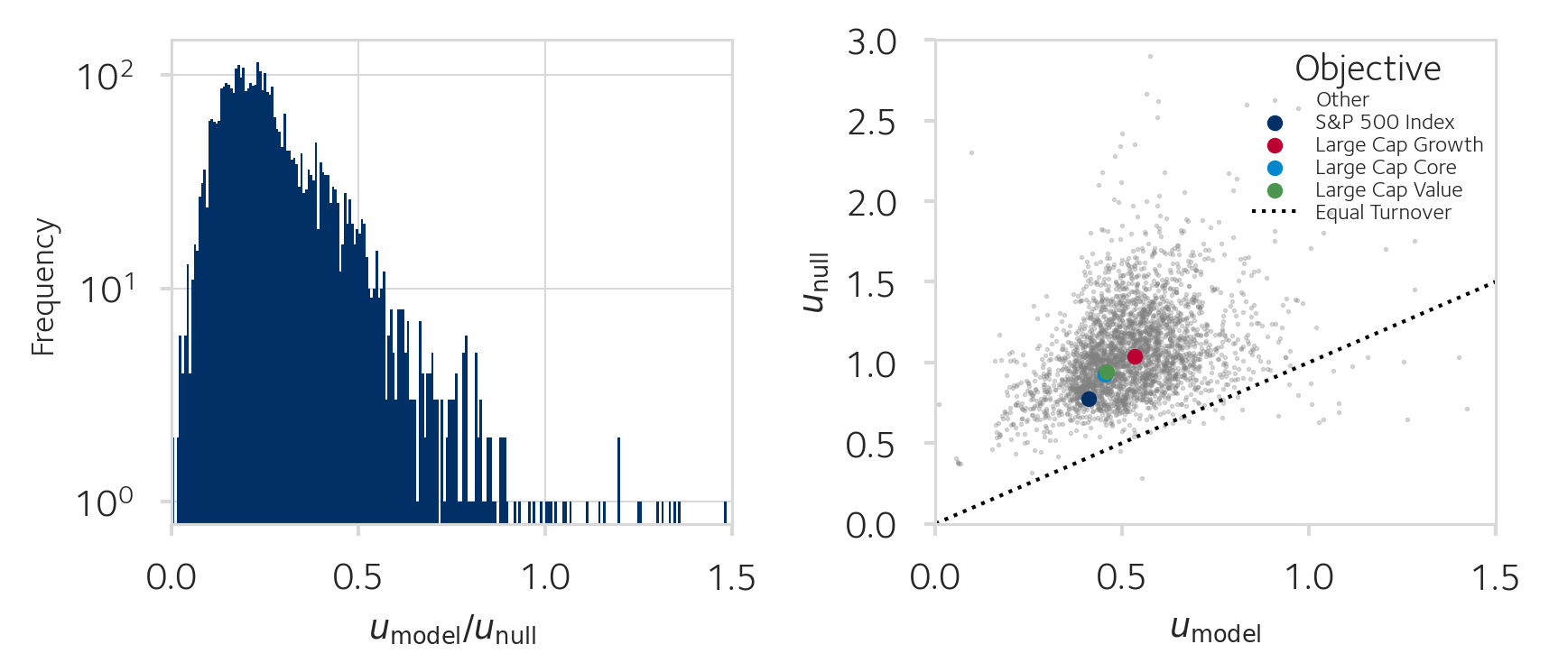
Nevertheless, in Appendix A we work out the statistical tests should we in the future want to compare more competitive models.
Analysis of Markowitz-Optimality
The average distance between the real-world portfolios and the Sharpe-ratio optimised portfolio with the same factor exposures is 0.18 Sharpe. The distance between the realised portfolios and the unconstrained Sharpe-optimised portfolio 0.52 Sharpe, being much larger, indicating that most portfolios are plausibly constrained in part by their factor exposures, but this does not preclude other possibilities, such as the optimisation for other portfolio aspects such as the minimisation of turnover rate, or the failure the maintain a Markowitz-optimal portfolio in dynamic market conditions, or the usage of a different window of historic data in the backtest that are used to estimate the parameters to the optimisation problem.
On average, fewer than one in ten portfolios outperforms random portfolios with the same factor characteristics at the 1% confidence level. In other words, in the aggregated If the fraction of portfolios that are optimised is 0.09 at the 1% confidence level, then we need to adjust our estimate down by 1% false positives to 8% of portfolios.
There is high heterogeneity among the portfolios. In Figure 1.5, we observe that not only those portfolios close to the efficient frontier are likely optimised, but that there are also portfolios further away from the efficient frontier that are likely optimised. This is because on some sets (universes) of stocks, it much harder to find a combination of weights that is optimal in risk-adjusted reward terms, and there a small perturbation may have large implications for the realised ex-post Sharpe ratio. Contrast this with for example a set of stocks that is highly similar in all attributes and returns: there it is not difficult to find an allocation that is close to optimal in terms of the Sharpe ratio.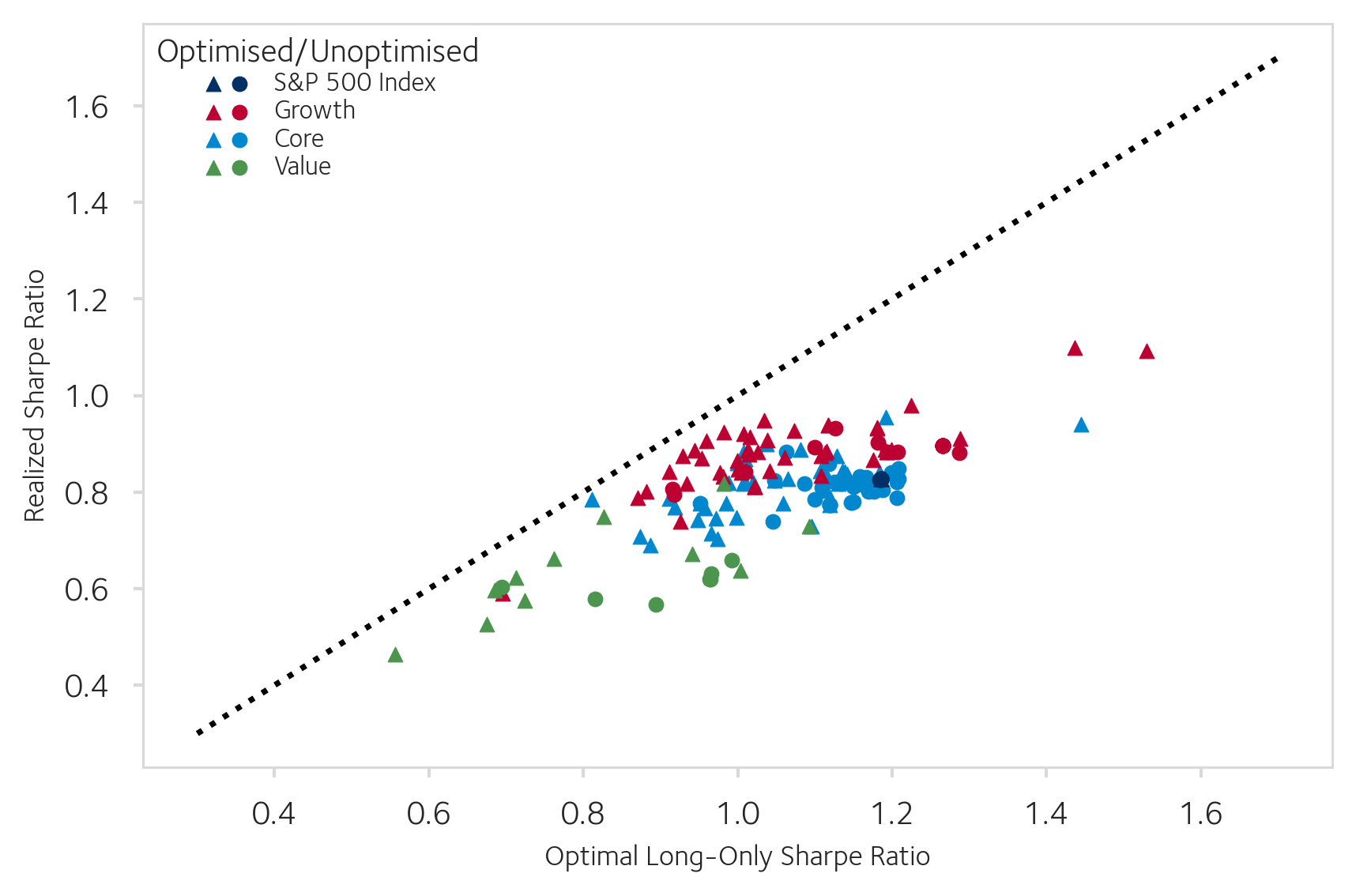
We plot in figure 1.5 the retrospective Sharpe ratios for the S&P 500 Index funds, Growth, Core and Value portfolios for January 2020. First, we observe that the sixty months preceding to this point in time resulted in good results for the buy and hold portfolios on average with a Sharpe ratio of 0.8. This period is also characterised by Value portfolios underperforming, and on the typical Growth portfolio outperforming the Core and Index funds slightly. Analysing the results, we see that index funds all sit at the same coordinate of a 0.8 realised Sharpe ratio, and our hypothesis test tells us no more of them are likely optimised beyond the false positive rate of 1%. This is expected, as the index funds target market capitalisation weights, and thus do not exploit expectations about future returns. Similarly, the Core portfolios in the vicinity of the index funds in terms of composition are rarely found to be optimised. Then, we also observe that near the Sharpe-ratio optimal boundary, nearly all portfolio pass the null-hypothesis test and are deemed to be optimised, and the more we move away from the boundary the less likely it is that portfolios pass the null-model test. There is however no sharp border between the two. This is because the universes of stocks are different between portfolios. For some sets of stocks, for example where the stocks are highly similar, it may be easy to land on a near-optimal allocation by chance. In such universes, the threshold for a portfolio to outperform the null model in the backtest is much higher, and so many portfolios are likely flagged as not being optimised. Conversely, if the universe of stocks is large and demands a complex combination of many non-zero positions, it may be very hard to arrive at an optimised portfolio by chance, and so a portfolio that is optimised does not necessarily have to be close to the optimality boundary in terms of the Sharpe distance.
The breakdown per prospectus objective for year-end 2019 is summarised in Table 1.3:
| Objective | Est. Percentage Optimised |
|---|---|
| S&P 500 | 0.0% |
| Growth (all market caps) | 56.3% |
| Core (all market caps) | 27.0% |
| Value (all market caps) | 55.5% |
| Income | 23.6% |
- This table lists the estimated percentage of portfolios that are likely risk-reward optimised, separated to the objective code as stated in the prospectus.
[]{#table:optimised_portfolios_percentages label=”table:optimised_portfolios_percentages”}
None of the S&P 500 index tracking funds appear to be optimising. This is not surprising, as the task of index funds is to track the index by market capitalisation weight, and except for the rare case where the optimal portfolio weights’ coincide with the market capitalisation weighted portfolio, the portfolio weights are likely to be different.
We learn that style portfolios in either the growth or the value category are most likely to optimise their portfolio. Core portfolios, which already have much overlap with S&P 500 index funds, don’t appear to optimise that often, which suggests that many core funds may not offer much beyond what an index-tracking fund does. Finally, income funds have also low likelihood of optimisation under our test. In our test using total returns, we do not account for the dynamics of distributions such as dividends separately. Therefore, it is possible that income funds design their portfolios with other objectives in mind, such as expectations about future dividend streams that are not easily captured in the risk-adjusted optimisation Markowitz framework.
Learning to Manage a Portfolio
We train the proposed neural network model from Section 1.3.4.1 on portfolios filtered for complete data (requirements in Section 1.2.2) and filtered to have a Lipper classification. Furthermore, we restrict the range to the dates from 2010 through 2022, as the data coverage after 2010 is complete and captures almost all major mutual funds. We fix the number of latent variables . We arrive at this number by giving the encoder at least eight variables to describe the risk-factor exposures for the portfolio: the idiosyncratic returns , market beta , and the six latent factors make up the first eight variables of the strategy. To this, we add an additional dimension for a returns-based description of the portfolio and a tenth variable for a turnover-based description. By partitioning the encoder so that the first eight latent variables can only be set by the part of the network observing the risk exposures and weights, we prevent the fusing of signals relating to the different tasks. This improves interpretation and prevents the signal of one task crowding out that of others, but comes at the theoretical cost of having reduced capacity in the latent representation compared when the signals are allowed to be mixed.
Style Representation
With one latent variable to describe the portfolios alpha and risk factor loadings, in theory there is just enough bandwidth to describe one important statistic of these variables, for example the mean factor exposure, but we can’t exclude the importance of higher moments of the distribution of exposures. In our experiment, however, we find that the information content in the portfolio weights as projected on the risk factor loadings is low, as when typically training the model the strategy encoder uses only six or seven out of eight available latent variables depending on random initialisation, as evidence by a constant output for these latent variables and zero gradients.
Of course, it is possible that the neural network encoder manages to summarise many important statistics by learning highly complicated correlations between portfolios. However, using simple linear analysis of the data we confirm this is likely not the case.
Take the tensor of weights at one point in time. We investigate the projection . An estimate for the effective number of factors is the of the distribution of contributions of each weighted factor to the total variance.
.
Computing this for each decade gives a range of Shannon entropies between , indicating that fewer than 8 factors contribute to the variance of the results. As with the variance explained for single stocks, for portfolios the market beta is most informative, explaining 25.6% of returns, followed by (16.4%), (15.5%), (11.2%).
Optimisation and Turnover
The final two latent variables are partitioned to explore the relationship between weights and historical returns , and the relative turnover rate .
Inspection of the two latent variables show that neither have high variation and are unlikely to make much difference in the resulting reconstructed allocation. The two latent variables are also highly correlated with an -squared of approximately 0.9, meaning that the neural network associates extreme scores on the Sharpe ratio with extreme scores on turnover. The direction of that relationship is not clear from the neural network, but investigating trends among the strategies as defined by Lipper gives insight. The two latent variables group together S&P 500 index funds and large cap core funds. Value funds overlap moderately with the two aforementioned types, and growth funds are separate and show the largest variation in values on the latent variables. This coincides with the real-world statistics, where growth funds tend to display larger volatility, higher factor drift and higher turnover rates.
Results on Anchor-Metrics
Recall, we introduced three losses that not only help anchor the generator and discriminator, but which are also easily interpretable by the practitioner as summary statistics of the performance of the model on a validation set. The summary statistics are Equations [equation:mean_exposure_regularization],[equation:sharpe_regularization],[equation:turnover_regularization]. These are summarised in Figure 1.4, where we present the summary statistics averaged over all funds in the given Lipper Class for January 2020.
| Lipper Class | |||
|---|---|---|---|
| S&P 500 Index | 6.2% | 0.141 | 9.4% |
| Value | 6.6% | 0.196 | 11.7% |
| Core | 7.9% | 0.171 | 11.4% |
| Growth | 9.0% | 0.163 | 13.1% |
| Income | 5.5% | 0.199 | 12.6% |
- This table compares the regularisation losses, breaking them by reference Lipper class. We observe that the strategy-modelling neural network performs better for index funds, where the regularisation losses are all lower than for other categories. Other results are more mixed, though value funds are often easily constructed, and growth funds are more difficult to replicate.
We summarise the regularisation losses for various classes, as a heterogeneity is observed in the performance of the model. As is mirrored in earlier experiments on factor exposure, turnover and optimisation, simple strategies such as the S&P 500 index strategy is easy to replicate, with the network obtaining the lowest losses. Again, more volatile strategies such as Growth strategies, which also show the largest variation in the data, are more difficult to replicate.
Note also that the relative weights of these losses is set rather arbitrarily to have the same standard error close to the end of training, whereas other schemes to set the weights may result in different outcomes, perhaps trading performance on one aspect for that in another, which we have not fully explored in this analysis.
GAN-based Unsupervised Strategy Learning
In Figure 1.6 we visualise the latent space of the strategy representation for funds with a reference Lipper classification. We will evaluate this qualitatively, as the connection between the latent space representation and the practical strategy of allocating the weights is complex.
The first eight latent variables are those we reserved for the encoder to encode information relating to factor exposures. As discussed before, there is excess capacity in the network, as we see a simple relation between the latter pairs and , which suggest that the network has unused degrees of freedom to capture additional information about the strategy. The fifth panel compares the latent dimension that encodes information about the weighted returns in the backtest and the dimension partitioned to capture information about the turnover rate . It is clear that these separately encoded aspects of the investment strategy correlate, primarily because the set of growth funds lies outside the main cluster. This suggests that these two latent variables could be picking up a common cause (or confounder): for example, it is known that growth stocks’ returns exhibit larger volatility that other stocks, causing growth funds’ returns to differ from other funds and also making it difficult to track a growth style exposure resulting in larger turnover. Alternatively, the correlation of these variables can be coincidental: growth funds could be optimising their portfolio differently independent of their turnover, and that information about optimising behaviour is abstractly encoded in such a way that it appears to correlate with their typically larger turnover.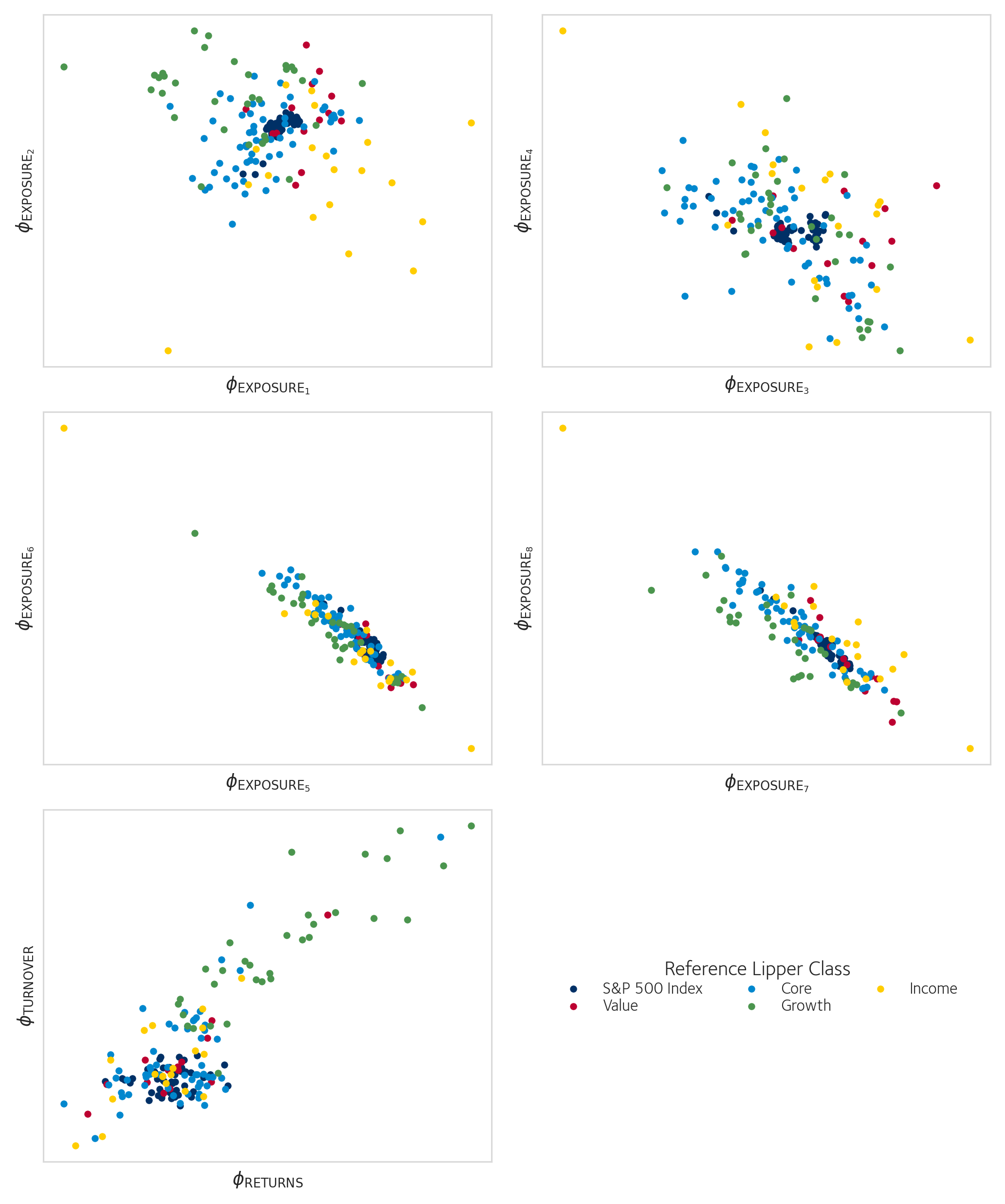
Conclusions
Fund managers exhibit coordination on stable factor exposures. Index funds, as expected, show the least drift, while growth-oriented funds exhibit the highest average drift. This indicates that maintaining stable exposure to growth-related factors is more challenging due to underlying volatility and market dynamics. The majority of portfolios deviate from the theoretical Sharpe-ratio optimal frontier. While some funds align closely with the efficient frontier, most portfolios appear influenced by constraints or objectives beyond pure risk-reward optimisation, such as turnover minimisation, liquidity considerations, or dynamic market conditions.
Analysis of intra-firm differences among growth and value funds suggests significant variation in how fund managers interpret and implement investment styles. This diversity underscores the importance of flexible models that accommodate heterogeneity across strategies.
The neural network model effectively captured key portfolio characteristics, such as risk-factor exposures and turnover. However, latent variables primarily summarised simple statistics rather than complex interdependencies, reflecting limited information content in observed portfolios beyond the average factor exposure. Growth funds display higher turnover and larger Sharpe-ratio variation compared to other classes. These differences are captured effectively in latent representations, suggesting that these metrics are fundamental to distinguishing growth strategies from other styles
Many of these features are computationally intensive to test at scale, as testing against a null model requires sampling from a complicated distribution that may be shaped by difficult-to-satisfy constraints. The GAN provides a framework for replicating investment strategies but foregoes easy interpretation. Regularisation terms based on Sharpe ratio, turnover, and factor exposures help stabilise training and guide the model toward realistic portfolio replication
Discussion
Interpretability remains a critical limitation, particularly for applications requiring transparency, such as regulatory settings. The GAN-based architecture demonstrated its usefulness in generating portfolio weights conditional on a given strategy. The discriminator’s learned criteria and latent space structure are difficult to interpret directly. Future work should explore better explainable models.
The monthly frequency of holdings data imposes significant limitations on reconstructing dynamic trading strategies. Higher-frequency data is invaluable. Alternatively, other data sources such as agent-based models could serve as sources for data. Using those models, the strategy encoder could learn pure-strategy archetypes, which when classifying real-world strategies would be mixed together in again a continuous classification.
Null-model testing revealed that while fund classifications are largely stable, distinctions between classes are less pronounced, and that there is much overlap in terms of the risk factor exposure for most Lipper classes of U.S. equities funds. Growth funds stand out as an exception, showing greater internal variability, but overall differences between classes lacked statistical significance. This suggests a need for richer datasets or more sophisticated models to capture subtle distinctions.
Because the number of observations per fund is quite limited with at most monthly portfolio snapshots, it is questionable that the strategy network can fully learn and generalise such complex operations as learning to Markowitz-optimise or target a specific volatility. Knowing that these aspects are almost universally tracked by real fund managers, these could perhaps be modelled as explicit components in the neural network.
Future studies could incorporate advanced metrics like maximum drawdown, skewness, or kurtosis to evaluate portfolios comprehensively. These metrics could better capture non-linear risk preferences or optimisations, and neural networks are suited to model these complicated aspects.
In conclusion, this chapter provides a foundation for understanding and replicating investment strategies using a combination of factor models, machine learning, and generative methods. Despite challenges in interpretability and data limitations, the methods developed here pave the way for more robust and nuanced analyses of portfolio management practices.
When it comes to classification, it appears there are few instances of an archetypal implementation of a strategy: under all factor models that the portfolio holdings data was tested, the different portfolios formed a continuum in factor space.
The VAE-based factor model nor the GAN-based neural network do not encode stocks and funds respectively, with the goal of matching the Lipper classification. Taking the mean exposures of a fund is closest in spirit to the approach taken by Lipper, and it is thus no surprise that the experiment of Section 1.3.1.2 (Table 1.2) yields such high similarity. What is surprising however is that so much structure remains visible in the unsupervised approach in Section 1.4.5. Particularly in Figure 1.6, in the first panel we see that the and separate the various classes well. The same variational methods that were applied to the factor model could in the future also be applied to regularise the layout of the latent space in this model, perhaps improving separation, and yielding better performance on unseen data.
The Lipper classes do serve as a useful reference and aid in implementation. This makes us reflect on using such established models as methods to make more advanced neural-networks more interpretable, by for example using them to construct archetypal or pure strategies that serve as a reference in the latent space. Perhaps neural networks operating on mixed modalities could construct explanations alongside the factor models and strategy classifications.
In essence, utility functions. ↩